Website Design Copyright 2026 © 耀登科技股份有限公司
All Rights Reserved. 網頁設計 by 覺醒設計
頻率選擇表面 (Frequency Selective Surface, FSS) 是一種由人工結構組成的表面材料,通常呈現平面或曲面的形式。它由規則排列的金屬圖案組成,這些圖案常見形狀包括環形、方形、十字形等幾何圖案,並以陣列方式分布在基板上。FSS 能夠精確調控特定頻段的電磁波,對某一頻率範圍內的電磁波實現選擇性反射、透過或吸收,功能類似濾波器。此技術廣泛應用於軍事、通訊、電子屏蔽以及智能建築等多個領域。
本教學範例將示範如何利用 Sim4Life 軟體,建模並模擬一種二維週期性圓形環陣列的頻率選擇表面(FSS)結構,進一步分析當平面電磁波入射時,該結構的反射係數特性。
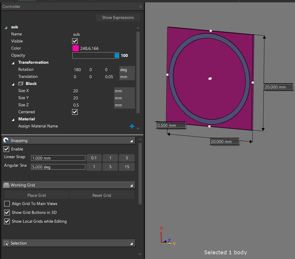
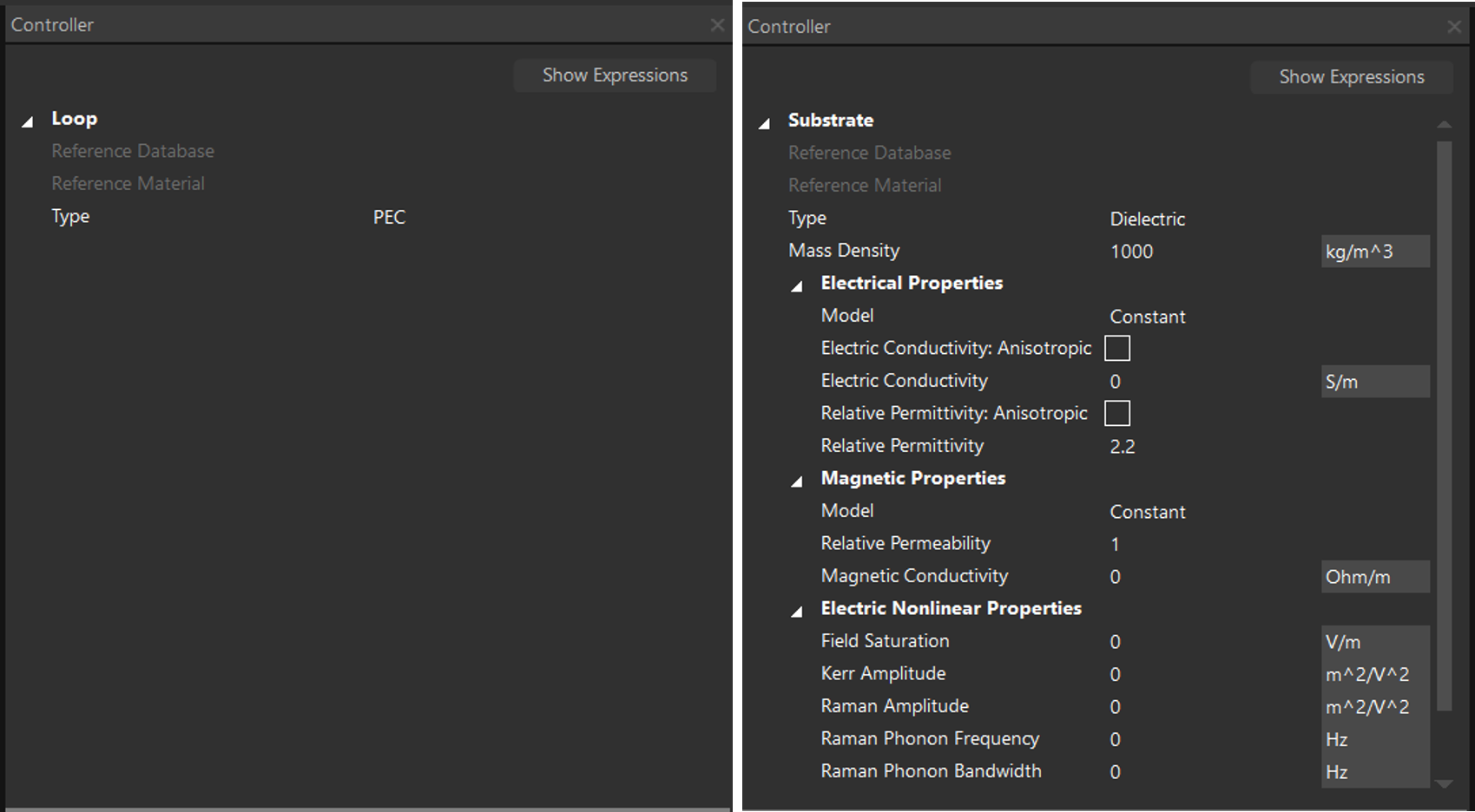
(1) 右圖顯示二維週期性圓環陣列頻率選擇表面的單元晶格(Unit cell)模型,晶格中由一個印刷的圓形導電環和一層薄基板所組成。我們在 Sim4Life 建模介面建立這個結構:
薄基板
圓環(貼附在薄基板上)
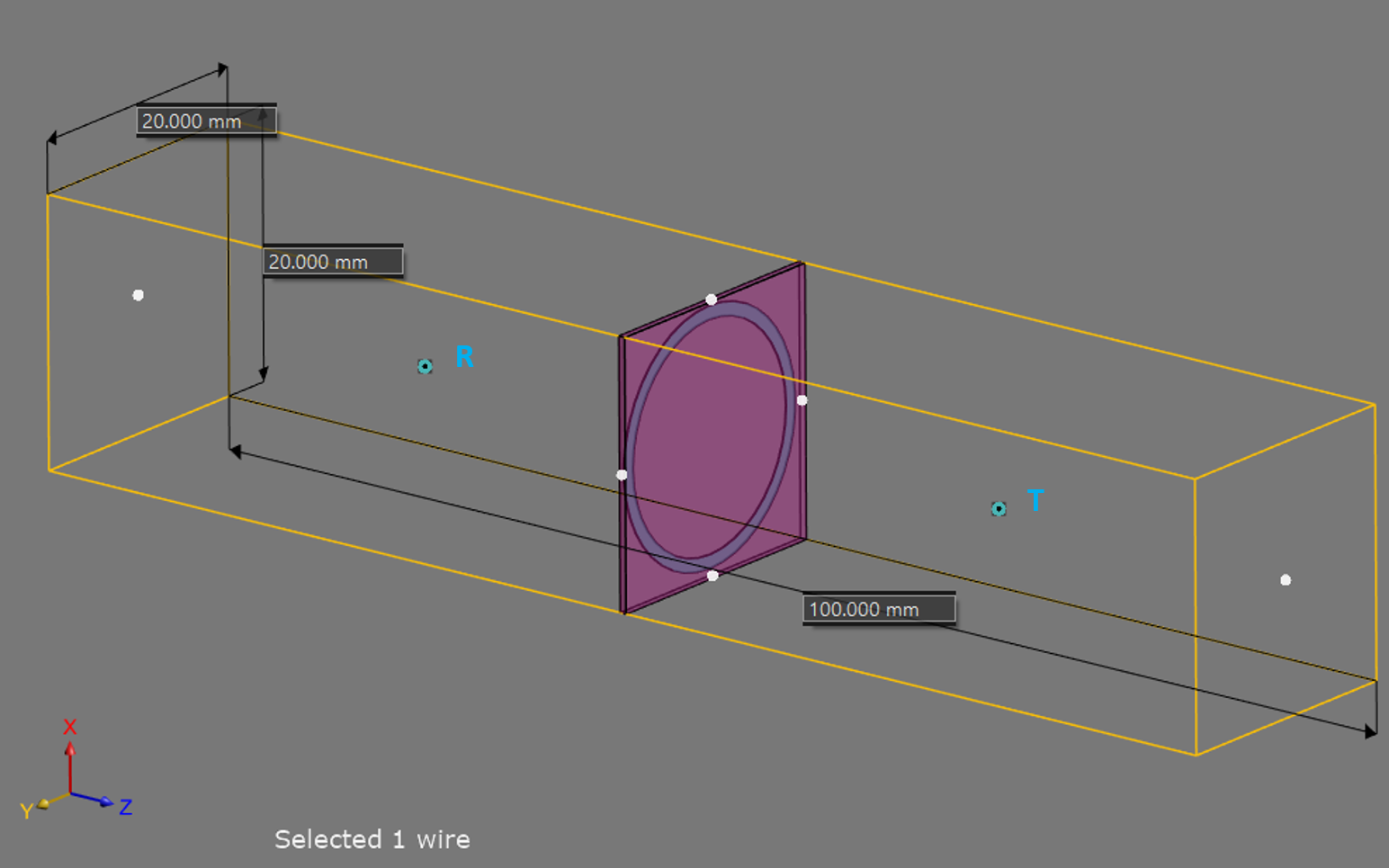
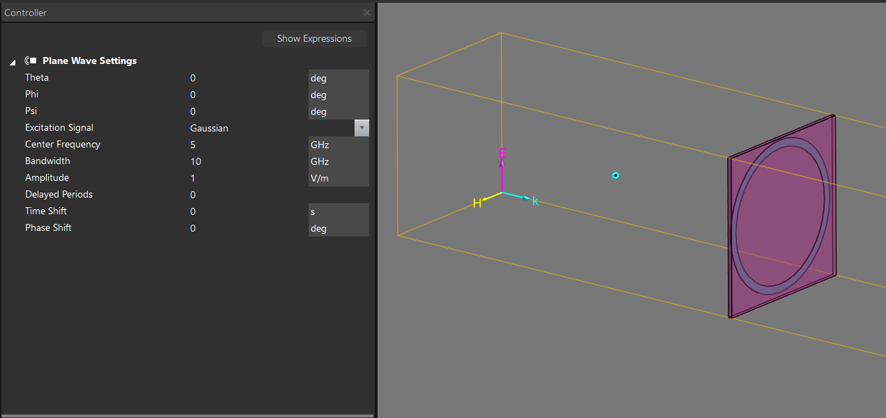
(2) 建立一個 Wire box 作為平面波源和兩個觀察點(T, R)紀錄平面波的穿透和反射。
Wire box
觀察點
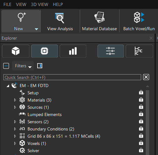
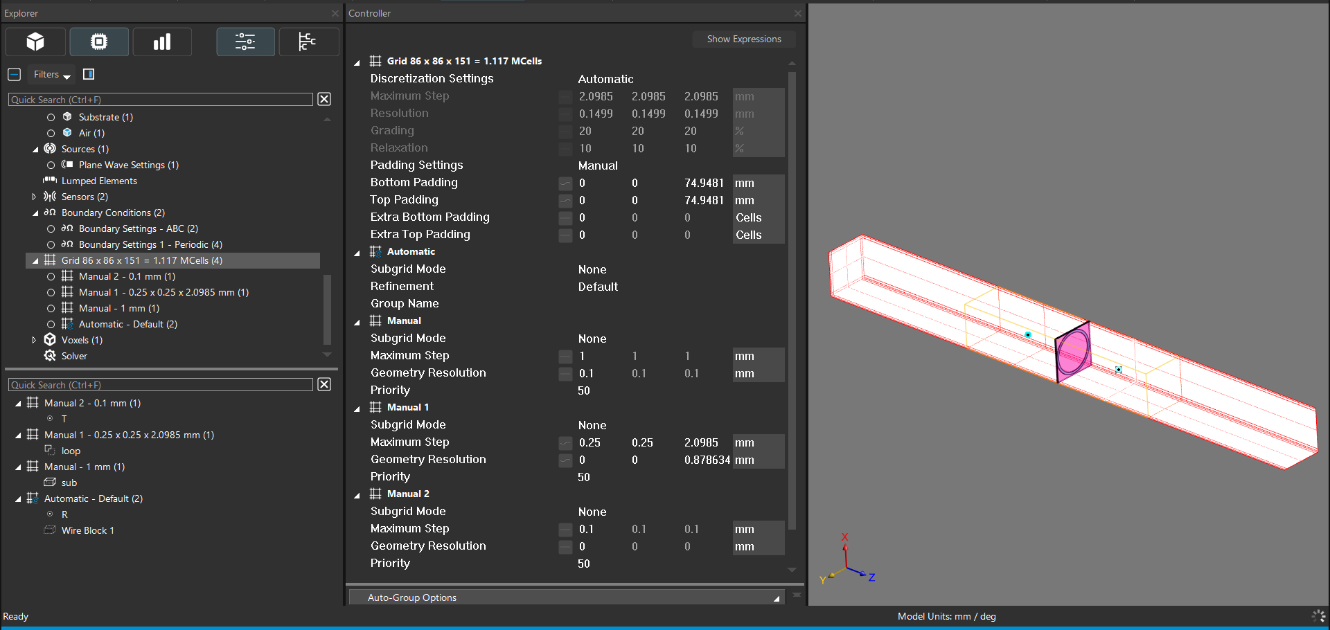
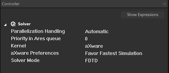
(1) 在 Simulation 介面建立 1 個 EM-FDTD Single 電磁求解器,用來模擬在 FSS 單元晶格存在時平面電磁波的行進。
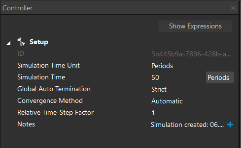
(2) 存在 FSS 單元晶格的模擬設定
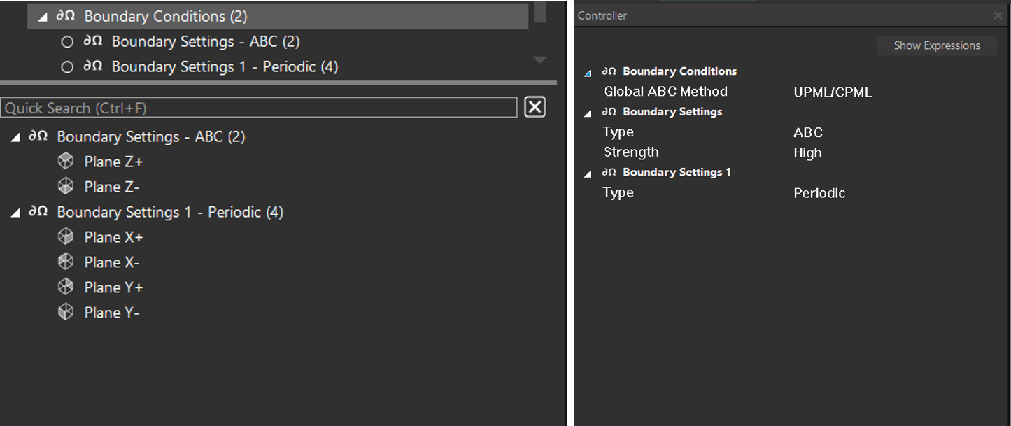
Plane X+/-、Y+/-、Z+/- 邊界條件型態示意圖:
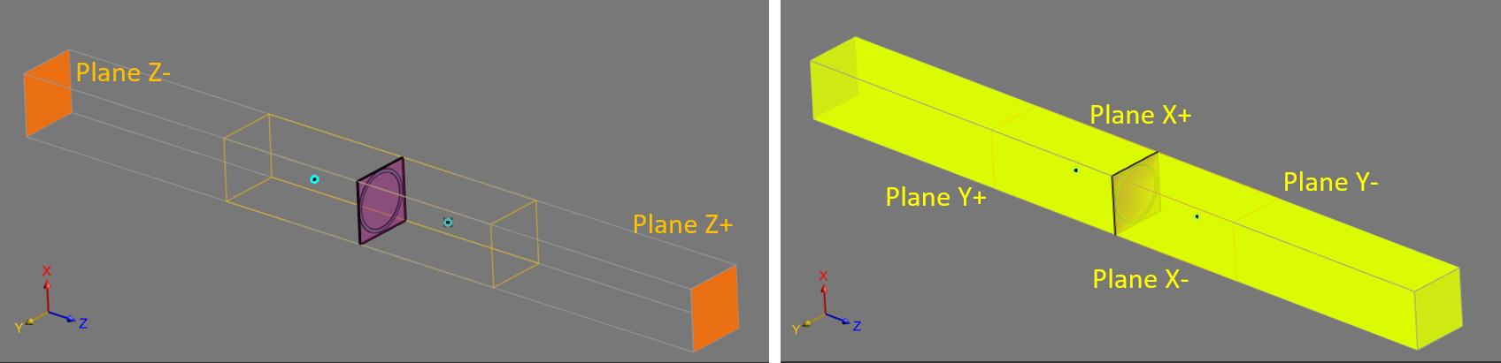
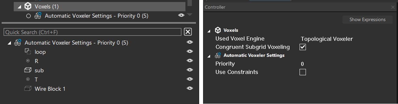
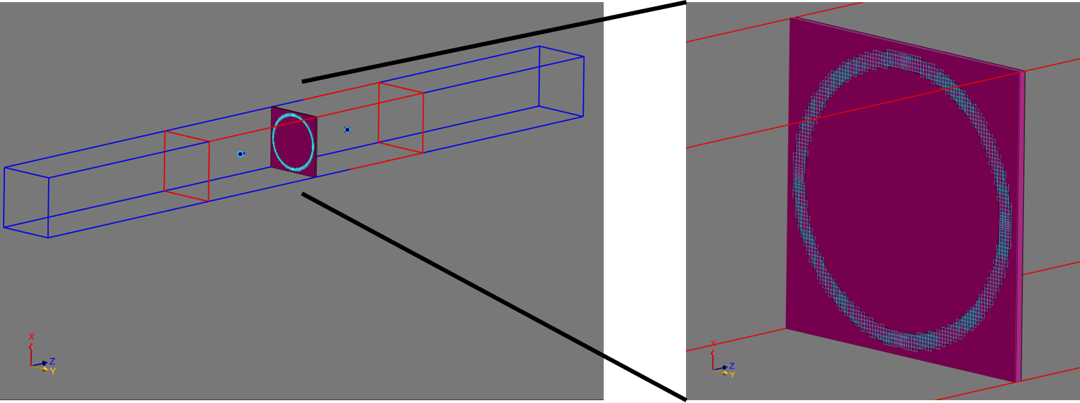
FSS 體素模型:
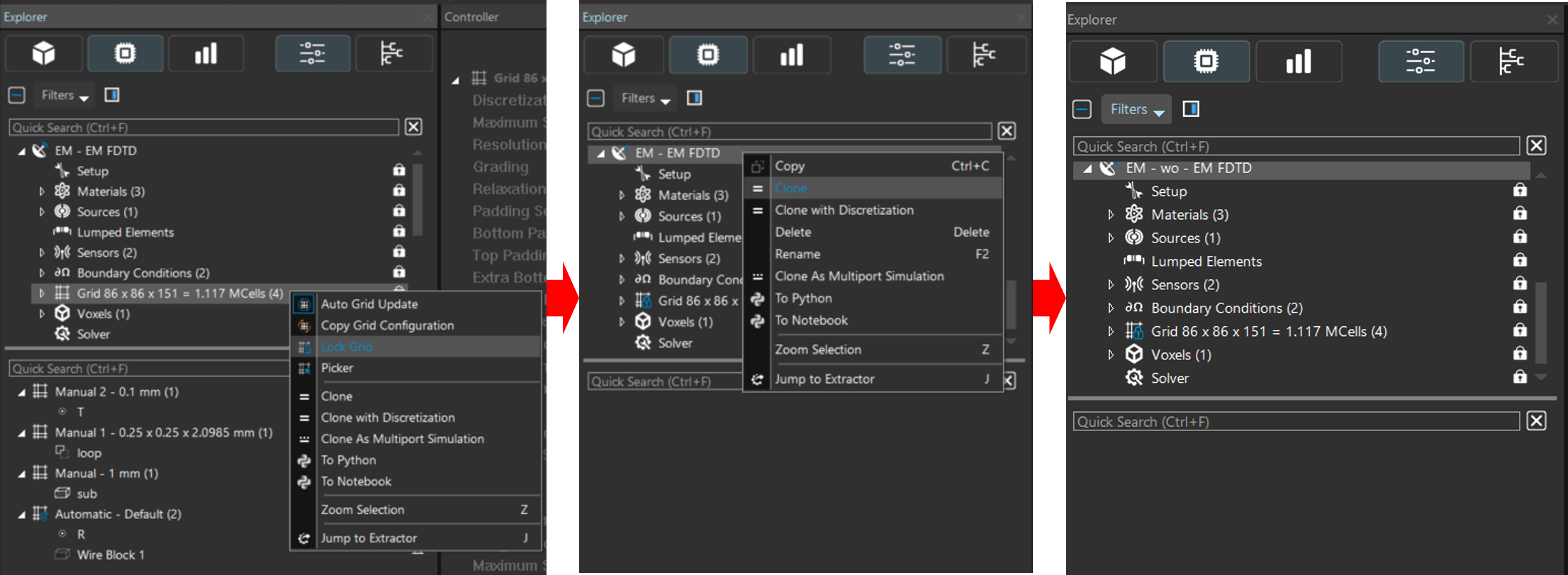
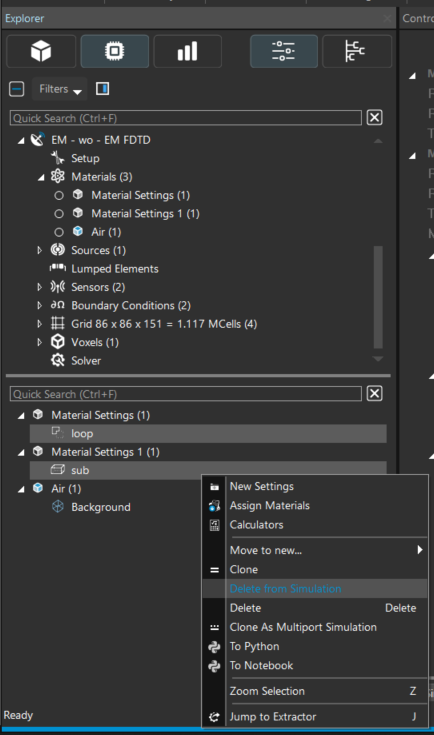
(3) 建立 1 個 EM-FDTD Single 電磁求解器,命名為 EM - wo,用來模擬在 FSS 單元晶格不存在時平面電磁波的行進
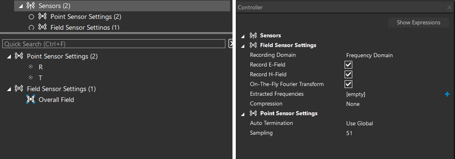
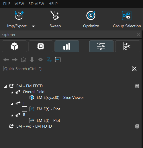
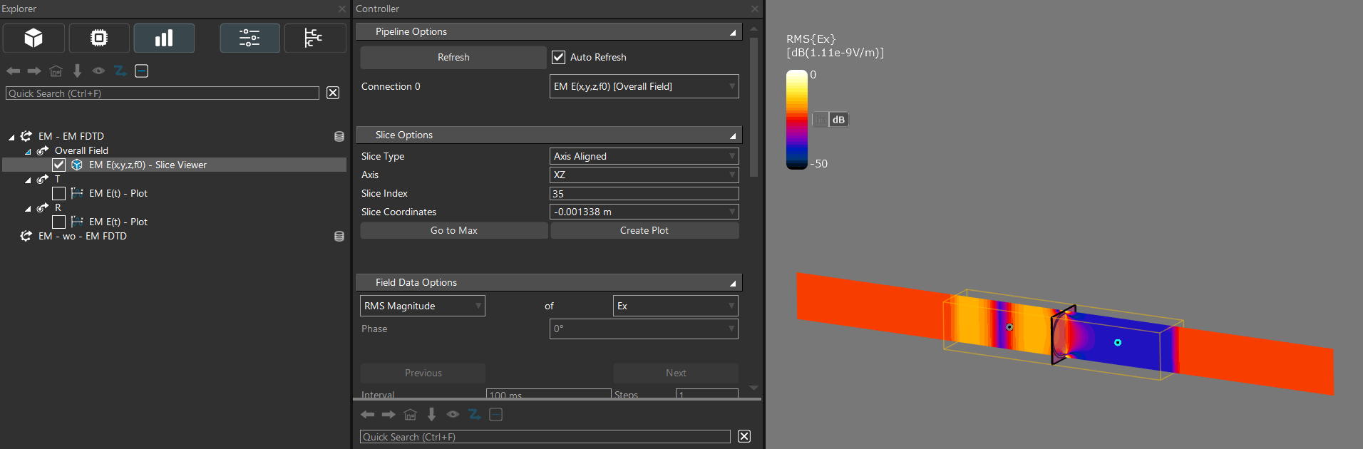
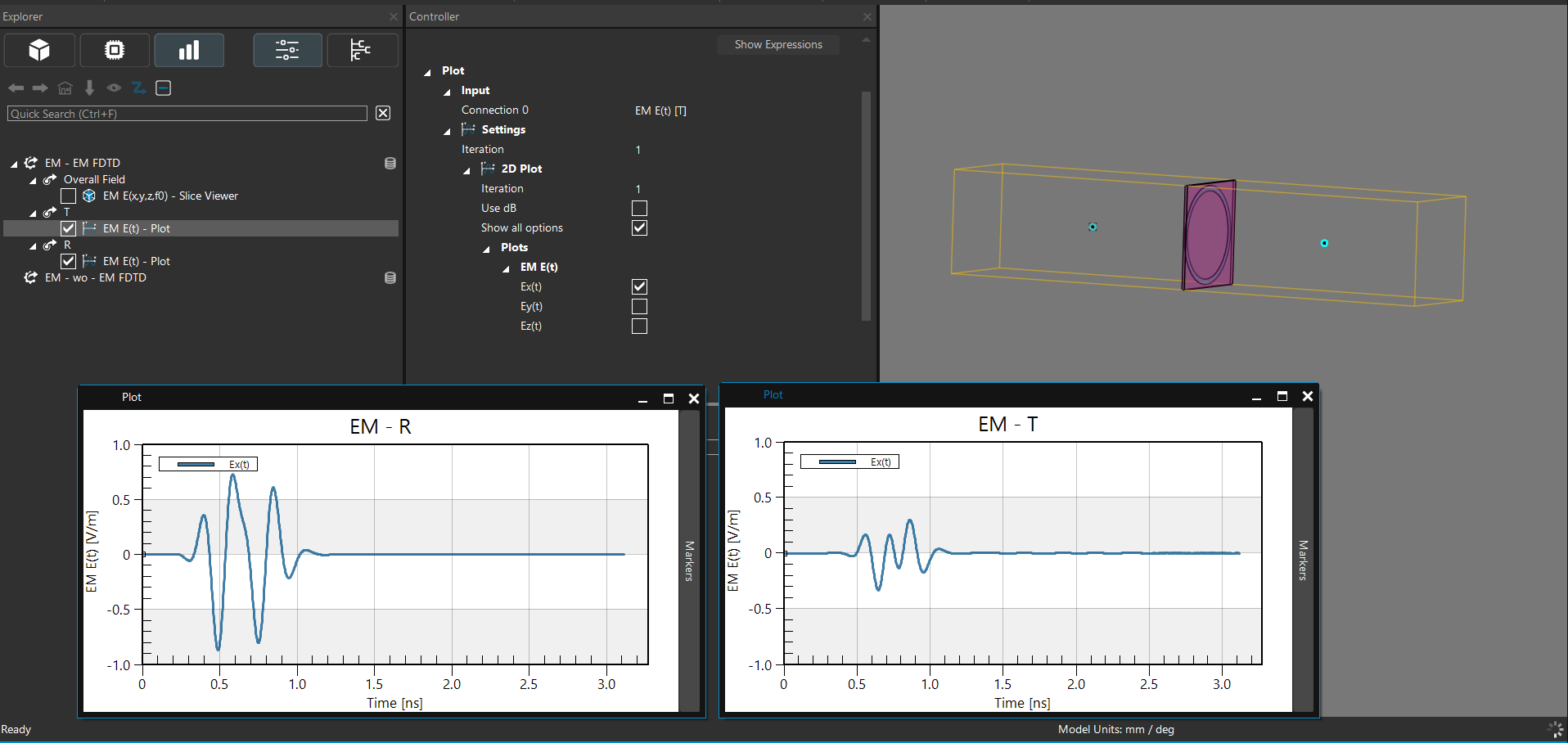
(1) 在後處理介面中會顯示兩個模擬結果文件夾(EM, EM - wo),我們可以點選 EM - EM FDTD,選擇 Overall field | EM E(x, y, z, f0),用工具欄位的 Viewer | Slice viewer 查看電場的分佈; 另外提取 R, T 兩個點感測器,選擇 EM E(t),用工具欄位的 Plot 查看電磁波反射與透射的訊號
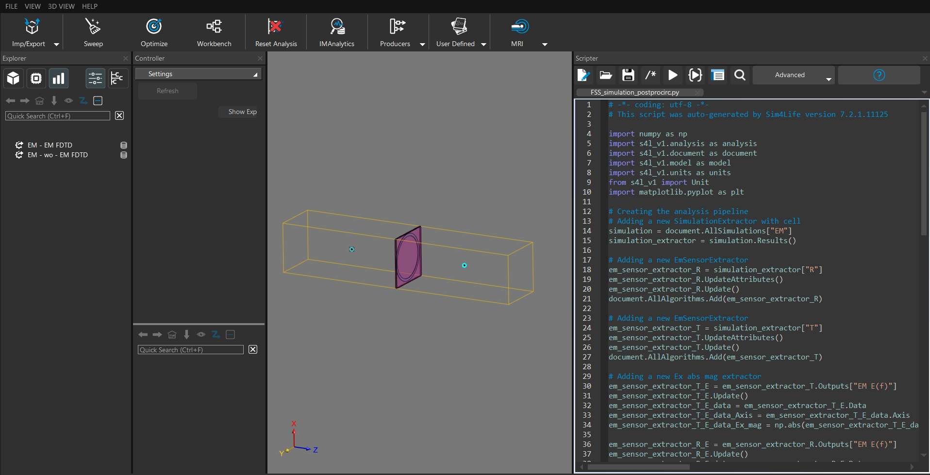
(2) 接下來我們開啟 Scripter 視窗,利用 Sim4Life 的 Python API 函式撰寫 python 腳本,由 R、T 兩個點感測器提取電場數據並計算 FSS 的 S 參數 (S11, S21)
範例程式碼:
# -*- coding: utf-8 -*-
# This script was auto-generated by Sim4Life version 7.2.1.11125

import numpy as np
import s4l_v1.analysis as analysis
import s4l_v1.document as document
import s4l_v1.model as model
import s4l_v1.units as units
from s4l_v1 import Unit
import matplotlib.pyplot as plt

# Creating the analysis pipeline
# Adding a new SimulationExtractor with cell
simulation = document.AllSimulations["EM"]
simulation_extractor = simulation.Results()

# Adding a new EmSensorExtractor
em_sensor_extractor_R = simulation_extractor["R"]
em_sensor_extractor_R.UpdateAttributes()
em_sensor_extractor_R.Update()
document.AllAlgorithms.Add(em_sensor_extractor_R)

# Adding a new EmSensorExtractor
em_sensor_extractor_T = simulation_extractor["T"]
em_sensor_extractor_T.UpdateAttributes()
em_sensor_extractor_T.Update()
document.AllAlgorithms.Add(em_sensor_extractor_T)

# Adding a new Ex abs mag extractor
em_sensor_extractor_T_E = em_sensor_extractor_T.Outputs["EM E(f)"]
em_sensor_extractor_T_E.Update()
em_sensor_extractor_T_E_data = em_sensor_extractor_T_E.Data
em_sensor_extractor_T_E_data_Axis = em_sensor_extractor_T_E_data.Axis
em_sensor_extractor_T_E_data_Ex_mag = np.abs(em_sensor_extractor_T_E_data.GetComponent(0))

em_sensor_extractor_R_E = em_sensor_extractor_R.Outputs["EM E(f)"]
em_sensor_extractor_R_E.Update()
em_sensor_extractor_R_E_data = em_sensor_extractor_R_E.Data
em_sensor_extractor_R_E_data_Axis = em_sensor_extractor_R_E_data.Axis
em_sensor_extractor_R_E_data_Ex_mag = np.abs(em_sensor_extractor_R_E_data.GetComponent(0))

# Adding a new SimulationExtractor without cell
simulation_wo = document.AllSimulations["EM - wo"]
simulation_extractor_wo = simulation_wo.Results()

# Adding a new EmSensorExtractor
em_sensor_extractor_R_wo = simulation_extractor_wo["R"]
em_sensor_extractor_R_wo.UpdateAttributes()
em_sensor_extractor_R_wo.Update()
document.AllAlgorithms.Add(em_sensor_extractor_R_wo)

# Adding a new EmSensorExtractor
em_sensor_extractor_T_wo = simulation_extractor_wo["T"]
em_sensor_extractor_T_wo.UpdateAttributes()
em_sensor_extractor_T_wo.Update()
document.AllAlgorithms.Add(em_sensor_extractor_T_wo)

# Adding a new Ex abs mag extractor
em_sensor_extractor_T_E_wo = em_sensor_extractor_T_wo.Outputs["EM E(f)"]
em_sensor_extractor_T_E_wo.Update()
em_sensor_extractor_T_E_data_wo = em_sensor_extractor_T_E_wo.Data
em_sensor_extractor_T_E_data_Axis_wo = em_sensor_extractor_T_E_data_wo.Axis
em_sensor_extractor_T_E_data_Ex_mag_wo = np.abs(em_sensor_extractor_T_E_data_wo.GetComponent(0))

em_sensor_extractor_R_E_wo = em_sensor_extractor_R_wo.Outputs["EM E(f)"]
em_sensor_extractor_R_E_wo.Update()
em_sensor_extractor_R_E_data_wo = em_sensor_extractor_R_E_wo.Data
em_sensor_extractor_R_E_data_Axis_wo = em_sensor_extractor_R_E_data_wo.Axis
em_sensor_extractor_R_E_data_Ex_mag_wo = np.abs(em_sensor_extractor_R_E_data_wo.GetComponent(0))

x_axis_GHz = em_sensor_extractor_T_E_data_Axis*1.e-9

S21 = em_sensor_extractor_T_E_data_Ex_mag/em_sensor_extractor_T_E_data_Ex_mag_wo
S21_dB = 20.*np.log10(S21)

S11_lst = []
for i in range(len(S21)):
    S11_lst.append(np.sqrt( 1. - S21[i]**2 ))
S11 = np.array(S11_lst)
S11_dB = 20.*np.log10(S11)

fig, ax = plt.subplots()
ax.plot(x_axis_GHz, S21_dB, label="S21", color='b')
ax.plot(x_axis_GHz, S11_dB, label="S11", color='r')
# ax.set_ylim([-25, 0])
ax.grid()
ax.legend()
ax.set_xlabel("Frequency [GHz]")
ax.set_ylabel("dB")

inputs = S21_dB
plot_viewer = analysis.viewers.PlotViewer(inputs=inputs)
plot_viewer.Plotter.ComplexOptions = plot_viewer.Plotter.ComplexOptions.enum.Real
plot_viewer.Plotter.ShowAll = True
plot_viewer.UpdateAttributes()
document.AllAlgorithms.Add(plot_viewer)
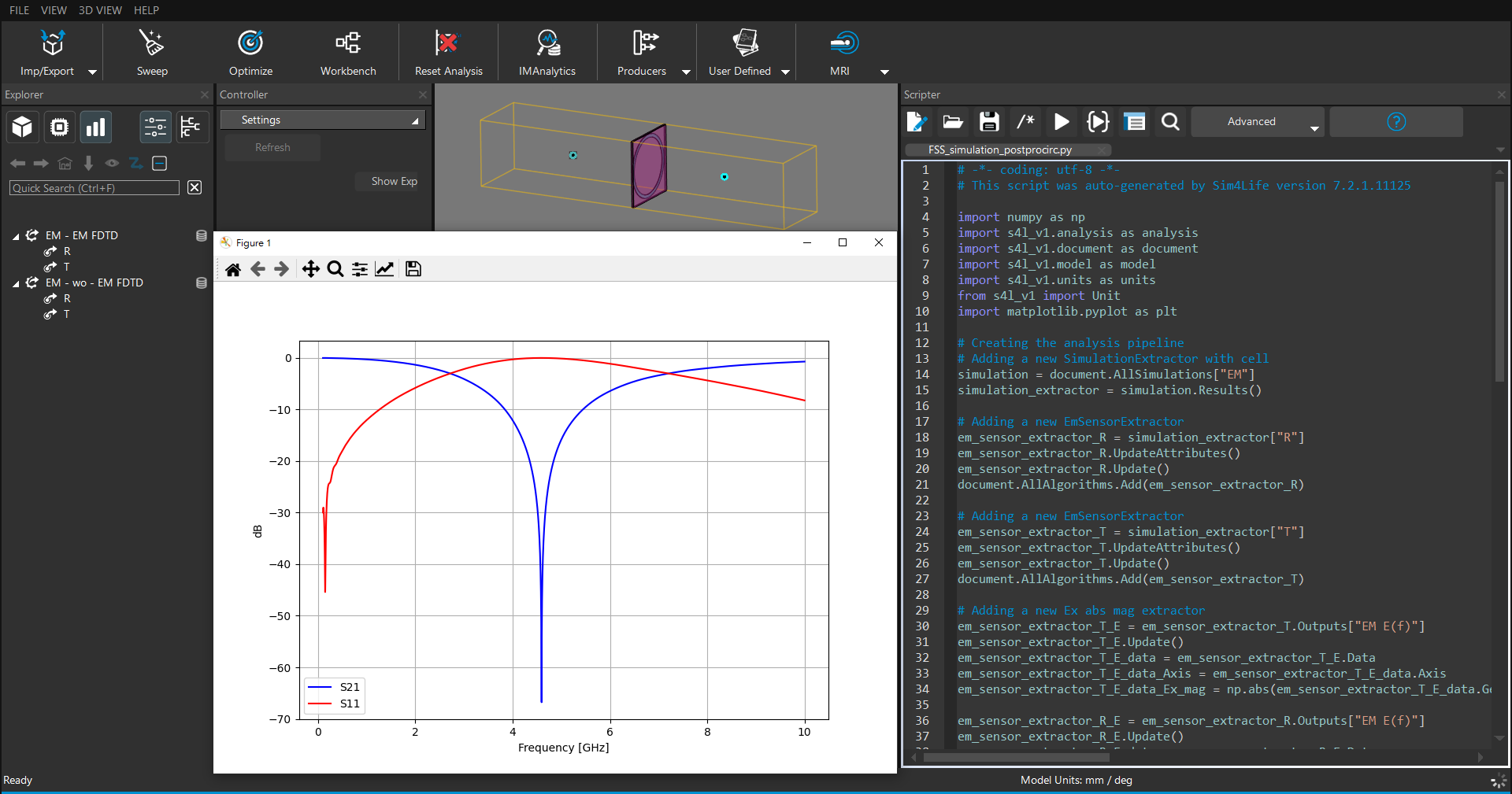
(3) 點選 Scripter 視窗的 Run 按鈕,執行腳本計算並生成一視窗顯示透射係數(S21)與反射係數(S11)圖形
依據歐盟施行的個人資料保護法,我們致力於保護您的個人資料並提供您對個人資料的掌握。
按一下「全部接受」,代表您允許我們置放 Cookie 來提升您在本網站上的使用體驗、協助我們分析網站效能和使用狀況,以及讓我們投放相關聯的行銷內容。您可以在下方管理 Cookie 設定。 按一下「同意」即代表您同意採用目前的設定,更多資訊請瀏覽 隱私權聲明。